.md .pdf

repository open issue

Contents

基础

机器学习分类

• 根据label的类型来分

  • Supervised learning algorithms： Learn a function that maps inputs to an output from a set of labeled training data.

    • Downside: getting labeled data is pretty costly. Hard to have clean labeled data.

    • 生成模型（常见的生成方法有LDA主题模型、朴素贝叶斯 算法和隐式马尔科夫模型等）：对判别式模型来说求得 \(P(Y \mid X)\), 对末见示例 \(X\), 根据 \(P(Y \mid X)\) 可以求得标记Y，即可以直接判别出来, 如上图的左边所示, 实际是就是直接得到了判别边界

    • 判别模型（ 常见的判别方法有SVM、LR等）：而生成式模型求得P(Y,X)，对于未见示例X，你要求出X与不同标记之间的联合概率分布，然后大的获胜，如上图右边所示，并没有什么边界存在

  • Unsupervised Learning: learn patterns from unlabeled data samples.

  • Reinforcement Learning: The computer employs trial and error to come up with a solution to the problem. To get the machine to do what the programmer wants, the artificial intelligence gets either rewards or penalties for the actions it performs. Its goal is to maximize the total reward.

  • Deep Learning: a class of ML algorithms that uses multiple layers to progressively extract higher-level features/abstractions from raw inputs.

    • 本质上也是create 很多features that you think is important

• 其他特定的学习方式

  • Active Learning：不是exposed to all training data, but we can ask for the label

    • 可以减少对label的依赖！

    • Create a human annotator, and makes tha ML ask for human to label

    https://en.wikipedia.org/wiki/Active_learning_(machine_learning)

    A learning algorithm can interactively query a user (or some other information source) to label new data points with the desired outputs

  • Self-supervised Learning: Trying to predict a label based on unlabeled data

    • Self-supervised learning techniques are generally used as pre-train tasks to generate labels for other downstream tasks.

      • e.g 补全单词预测——因为补全句子这种你用来补全的context words也不算labeled

      • word2vec，autoencoder这类明明没标签却能够造出目标函数，使用凸优化方法求解，无中生有

    • The learning model trains itself by leveraging one part of the data to predict the other part and generate labels accurately. In the end, this learning method converts an unsupervised learning problem into a supervised one

    • 区分定义

      • Self-supervised learning vs semi-supervised learning：自监督是完全没标签，半监督其实就是有部分标签的时候带了一些数据生产规则的有监督

        • Semi-supervised learning uses manually labeled training data for supervised learning and unsupervised learning approaches for unlabeled data to generate a model that leverages existing labels but builds a model that can make predictions beyond the labeled data.

          • 一个semi-supervised的例子：简单自训练**（simple self-training）：用有标签数据训练一个分类器，然后用这个分类器对无标签数据进行分类，这样就会产生伪标签（pseudo label）或软标签（soft label），挑选你认为分类正确的无标签样本（此处应该有一个挑选准则），把选出来的无标签样本用来训练分类器。

        • Self-supervised learning relies completely on data that lacks manually generated labels.

      • Self-supervised learning vs unsupervised learning：自监督的目标是监督学习，无监督不是

        • Self-supervised learning is similar to unsupervised learning because both techniques work with datasets that don’t have manually added labels. In some sources, self-supervised learning is addressed as a subset of unsupervised learning. However, unsupervised learning concentrates on clustering, grouping, and dimensionality reduction,

        • while self-supervised learning aims to draw conclusions for regression and classification tasks.

      • Hybrid Approaches vs. Self-supervised Learning：自监督学习和人类混合的差别是自监督是全自动的

        • There are also hybrid approaches that combine automated data labeling tools with supervised learning. In such methods, computers can label data points that are easier-to-label relying on their training data and leave the complex ones to humans. Or, they can label all data points automatically but need human approval.

        • In self-supervised learning, automated data labeling is embedded in the training model. The dataset is labeled as part of the learning processes; thus, it doesn’t ask for human approval or only label the simple data points.

  • Transfer Learning：pre-trained models are used as the starting point on computer vision and natural language processing tasks

模型的评测指标

metric主要用来评测机器学习模型的好坏程度，不同的任务应该选择不同的评价指标。分类，回归和排序问题应该选择不同的评价函数。

Evaluation Metrics

• Evaluation metrics are generally used to measure the performance of an ML model.

• Evaluation metrics indicate how well the models would do when deployed

• The choice of metrics is very task-specific and determines what the model learns

  • can direct your model to learn specific things based on the evaluation metric

• It is important to know what you are willing to trade off when training ML models for a task

回归指标

• 平均绝对误差(MAE)，又称L1范数损失：

  \[MAE=\frac{1}{n}\sum_{i=1}^{n}|y_i-\hat{y}_i|\]

  • MAE虽能较好衡量回归模型的好坏，但是绝对值的存在导致函数不光滑，在某些点上不能求导，

  • 可以考虑将绝对值改为残差的平方，这就是均方误差。

• 均方误差(MSE)，又被称为 L2范数损失 。

  \[M S E=\frac{1}{n} \sum_{i=1}^{n}\left(y_{i}-\hat{y}_{i}\right)^{2}\]

  • 由于MSE与我们的目标变量的量纲不一致，为了保证量纲一致性，我们需要对MSE进行开方 得到RMSE

  • Outlier多时会被push得非常高, MSE会让model去predict outlier right 所以要么tune outlier再用MSE，要么就用MAE

• 均方根误差(RMSE)

  \[RMSE=\sqrt{\frac{1}{n}\sum_{i=1}^{n}(y_i-\hat{y}_i)^2} \]

• \(R^{2}\)又称决定系数，表示反应因变量的全部变异能通过数学模型被自变量解释的比例

  \[R^{2} =1-\frac{\sum^n_{i}\left(y_{i}-\hat{y}\right)^{2} / n}{\sum^n_{i}\left(y_{i}-\bar{y}\right)^{2} / n}=1-\frac{M S E}{\operatorname{Var}} \]

  • \(y\)表示实际销量, \(\hat{y}\)表示预测销量, \(\bar{y}\)表示实际销量的均值, \(n\)表示样本数, \(i\)表示第\(i\)个样本, \(Var\)表示实际值的方差，也就是销量的变异情况。

  • \(R2_{score}\)越大，模型准确率越好。

  • \(MSE\)表示均方误差，为残差平方和的均值,该部分不能能被数学模型解释的部分,属于不可解释性变异。

    • 因此： $\(可解释性变异占比 = 1-\frac{不可解释性变异}{整体变异}= 1-\frac{M S E}{\operatorname{Var}} = R2_score \tag{5} \)$

• Mean Absolute Percentage Error (MAPE): \(\frac{100}{n} \sum_{i=1}^{n} \mid \frac{y_{i}-\hat{y}_{i}}{y_{i}}\)，特点是跟value本身大小也有关系

  • Intuition：y范围很大时候 大y当然会带来大的error, 所以不make sense

分类指标

分类

• Threshold-based metrics

  • Classification Accuracy

  • Precision, Recall & F1-score

• Ranking-based metrics

  • Average Precision (AP)

  • Area Under Curve (AUC)

准确率和错误率

\[Acc(y,\hat{y})=\frac{1}{n}\sum_{i=1}^{n}y_i=\hat{y_i} \]

\[ Error(y, \hat{y})=1-acc(y,\hat{y}) \tag{7} \]

• Acc与Error平等对待每个类别，即每一个样本判对 (0) 和判错 (1) 的代价都是一样的。

• 使用Acc与Error作为衡量指标时，需要考虑样本不均衡问题以及实际业务中好样本与坏样本的重要程度。

Confusion Matrix / 评价指标

对于二分类问题,可将样例根据其真是类别与学习器预测类别的组合划分为

• 真正例(true positive, TP):预测为 1，预测正确，即实际 1

• 假正例(false positive, FP):预测为 1，预测错误，即实际 0

• 真反例(ture negative, TN):预测为 0，预测正确，即实际 0

• 假反例(false negative, FN):预测为 0，预测错误，即实际 1

通常把minority当作Positive : Minority class is considered positive as best practice——因为希望learn minority class well（如果要learn majority class就直接预测大多数就好了）

• 刚刚的$\(Accuracy=\frac{\sum_{i=1}^{n} I_{\hat{y_{i}}=y_{i}}}{n} = \frac{\colorbox{#eaf1f5}{TN+TP}}{TN+TP+FP+FN}\)$

  • could be misleading in case of imbalance datasets

  • accuracy paradox: higher the accuracy does not necessarily mean a better model.

    • 比如风控直接说大家都是正常的 accuracy一样很高

Normalize by y_true	Normalize by y_pred
True Positive Rate / Recall / Sensitivity = $\(\frac{\colorbox{#c9e8ee}{TP}}{\colorbox{#c9e8ee}{TP}+FN}=\frac{TP}{所有Positive样本}\)\(：the fraction of relevant instances that were retrieved <br> False Positive Rate = \)\(\frac{\colorbox{#d9ed8a}{FP}}{\colorbox{#d9ed8a}{FP}+TN}=\frac{FP}{所有Negative样本}\)$	Precision= $\(\frac{\colorbox{#c39dc6}{TP}}{\colorbox{#c39dc6}{TP}+FP}=\frac{TP}{所有Positive预测}\)$：the fraction of relevant instances among retrieved instances
能把癌症的人中的多少检测出来	判定成spam中有多少是实锤，下结论的时候有多precise
$\(\text{F1-Score} =2 \times \frac{\text { Precision*Recall }}{\text { Precision+Recall }}\)$：harmonic mean of precision & recall 当两边都在意的时候用F1！

Precision VS Recall

• 准确率（查准率） Precision：分类器预测的正样本中预测正确的比例，取值范围为[0,1]，取值越大，模型预测能力越好。 $\( P=\frac{TP}{TP+FP} \tag{8} \)$

• 召回率（查全率）Recall：Recall 是分类器所预测正确的正样本占所有正样本的比例，取值范围为[0,1]，取值越大，模型预测能力越好。 $\( R=\frac{TP}{TP+FN} \tag{9} \)$

• F1 Score：Precision和Recall 是互相影响的，理想情况下肯定是做到两者都高，但是一般情况下Precision高、Recall 就低， Recall 高、Precision就低。为了均衡两个指标，我们可以采用Precision和Recall的加权调和平均（weighted harmonic mean）来衡量，即

  \[ \frac{1}{F_1}=\frac{1}{2} \cdot (\frac{1}{P}+\frac{1}{R}) \tag{10} $$, $$ F_1=\frac{2*P*R}{P+R} \tag{11} \]

• Averaging Metrics

  • \[\text{Macro Recall} = \frac{1}{|L|} \sum_{l \in L} R\left(y_{l}, \hat{y}_{l}\right)\]

    Average over recall per class equally ⇔ \(\text{Balanced Accuracy}= \frac{1}{2} \left(\frac{T P}{T P+F N}+\frac{T N}{T N+F P}\right)\)

  • \[\text{Weighted Recall}= \frac{1}{n} \sum_{l \in L} n_{l} R\left(y_{l}, \hat{y}_{l}\right)\]

    Weighted average (by class size) over recall per class ⇔ Accuracy

    • Imbalanced 的数据不用！不然会give a higher weight to the majority class.

计算举例：

• 全局：$\(Accuracy = \frac{23+2184}{23+2184+3+27} = 0.9865\)$

• Minority Class：

  • \[Recall = \frac{23}{23+27} = 0.46\]
  • \[Precision = \frac{23}{23+3} = 0.8846\]
  • \[F1\text{-}score = 2 \times \frac{0.8846 * 0.46}{0.8846 + 0.46} = 0.60526\]

• Averaging Metrics:

  • \[\begin{split}\begin{aligned} \text{Macro Recall} &= \frac{1}{2} (\frac{23}{23+27} + \frac{2184}{2184+3})= 0.7293 \\ &= \text{Balanced Accuracy} \end{aligned}\end{split}\]
  • \[\begin{split}\begin{aligned} \text{Weighted Recall} &= \frac{1}{2184+3+27+23} ((23+27) \times \frac{23}{23+27} + (2184+3) \times \frac{2184}{2184+3})) \\ &= \frac{23+2184 }{2184+3+27+23} = 0.9865\\ &= \text{Accuracy} \end{aligned}\end{split}\]

Metric Choosing的问题

原则：

• Problem-specific

• Balanced accuracy better than accuracy (most of the times)

• Cost associated with misclassification

两种场景：

场景	第一类错误（Reject True H0｜拒真｜FP）成本高	第二类错误（Accept False H0｜取伪｜FN）成本高
Metric	Choose precision $\(=\frac{TP}{TP+\colorbox{#a8b6e0}{FP}}\)$	Choose recall$\(=\frac{TP}{TP+\colorbox{#a8b6e0}{FN}}\)$
例子	Predicting an email as spam when it is not (false positive) has higher cost than predicting email as not spam “邮件False Positive第一类错误成本高，要非常小心precisely地给Positive预测，所以预测positive里面的TP要高⇒precision要高”	Predicting that an individual has no cancer when he/she has cancer (false negative) is far more costlier than the other way round “癌症False Negative第二类错误成本高，要尽量recall回所有的Positive=1 sample⇒recall要高”
做法	提高threshold：让每个y_pred_positive都是很sure的结果，牺牲recall但更加precise	降低threshold：多召回多预测出positive（predict negative的时候我非常sure），可以牺牲precision但提高recall y_true_positive的占比

曲线指标

Receiver Operating Curve (ROC) ⇒ Area Under Curve (AUC)

• 定义：ROC全称是”受试者工作特征”(Receiver Operating Characteristic)曲线，ROC曲线为 FPR 与 TPR 之间的关系曲线，这个组合以 FPR 对 TPR，即是以代价 (costs) 对收益 (benefits)，显然收益越高，代价越低，模型的性能就越好。

  • y 轴为真阳性率（TPR）（正样本Recall）：在所有的正样本中，分类器预测正确的比例

    \[ TPR=\frac{TP}{TP+FN} \tag{12} \]

  • x 轴为假阳性率（FPR）（负样本的1-recall）：在所有的负样本中，分类器预测错误的比例

    \[ FPR=\frac{FP}{TN+FP} \tag{13} \]

• 绘制过程：对有限个(真正例率,假正例率)坐标对：

  • 给定\(m^+\)个正例和\(m^-\)个反例,根据学习器预测结果对样例进行排序,然后将分类阈值设为最大,此时真正例率和假正例率都为0,坐标在(0,0)处,标记一个点.

  • 将分类阈值依次设为每个样本的预测值,即依次将每个样本划分为正例.

  • 假设前一个坐标点是(x,y),若当前为真正例,则对应坐标为\((x,y+\frac{1}{m^+})\), 若是假正例,则对应坐标为\((x+\frac{1}{m^-}, y)\)

  • 线段连接相邻的点.

• AUC：对于二分类问题，预测模型会对每一个样本预测一个得分s或者一个概率p。 然后，可以选取一个阈值t，让得分s>t的样本预测为正，而得分s<t的样本预测为负。 这样一来，根据预测的结果和实际的标签可以把样本分为4类,则有混淆矩阵：

  • 随着阈值t选取的不同，这四类样本的比例各不相同。定义真正例率TPR和假正例率FPR为： $\( \begin{array}{l} \mathrm{TPR}=\frac{\mathrm{TP}}{\mathrm{TP}+\mathrm{FN}} \ \mathrm{FPR}=\frac{\mathrm{FP}}{\mathrm{FP}+\mathrm{TN}} \end{array} \tag{14} \)$ 随着阈值t的变化，TPR和FPR在坐标图上形成一条曲线，这条曲线就是ROC曲线。 显然，如果模型是随机的，模型得分对正负样本没有区分性，那么得分大于t的样本中，正负样本比例和总体的正负样本比例应该基本一致。

  • 实际的模型的ROC曲线则是一条上凸的曲线，介于随机和理想的ROC曲线之间。而ROC曲线下的面积，即为AUC！

  • 这里的x和y分别对应TPR和FPR，也是ROC曲线的横纵坐标。 $\( \mathrm{AUC}=\int_{t=\infty}^{-\infty} y(t) d x(t) \tag{15} \)$

• 端点解读：

  

  • (1, 1)当recall (y轴的True Positive Rate)为1的时候，相当于召回全部正样本，类似threshold=0.01，那么这个时候所有的负样本都给你搞成Positive了没有TN，False Positive Rate = $\(\frac{\colorbox{#d9ed8a}{FP}}{\colorbox{#d9ed8a}{FP}+TN}=\frac{FP}{所有Negative样本}=\frac{所有Negative样本}{所有Negative样本}=1\)$

  • （0， 0）当recall (y轴的True Positive Rate)为0的时候，相当于什么正样本都不召回，类似threshold=0.99，那么这个时候根本没有错的Positive，False Positive Rate = $\(\frac{\colorbox{#d9ed8a}{FP}}{\colorbox{#d9ed8a}{FP}+TN}=\frac{FP}{所有Negative样本}=\frac{0}{所有Negative样本}=0\)$

Precision-Recall (PR) Curve

• A precision-recall curve shows the relationship between precision and recall at every cut-off point.

• Visualize effect of selected threshold on performance.

• （0， 1）当recall为0的时候，相当于没有一个正样本被召回， ⇒全部预测不是Fraud(Negative)了，也就没有错误的Positive，因此 $\(precision=\frac{TP}{TP+0}=1\)$

• （1， 0.93）当recall为1的时候，相当于我为了把所有正样本召回，threshold为0⇒我全部当Fraud打(预测Positive)，那么这时候毫无precise可言，因此 $\(precision=\frac{TP}{n}=precision_{min}\)$

对比

首先，两个都是both are ranking metrics：如果一个模型预测的probability是之前的一半，AUC和AP都不会改变！log-loss之类的才会改变

• Precision-Recall PR Curve ⇒ Average Precision(AP)

  • 好处是imbalance datasets表现更好make more sense： In case of imbalance datasets, AP is a better estimate indicative of model

    • AUC will still be very high even the model is bad! 没给你true picture：主要是AUC曲线横坐标是False Positive Rate也就是FP/所有负样本，分母是很大的，但TN没有价值（比如正确预测一个贷款的人不会违约）

      

• Receiver Operating Curve(ROC) ⇒ Area Unver ROC (AUROC / AUC)

  • AUROC measures whether the model is able to rank positive examples higher than negative samples

  • 根据probability来rank prediction：

    • 如果全（就是正确地把positive都放上面）的情况下：从threshold=1 recall=0 慢慢下降threshold的过程中不会有False Positive出现，所以在FPR=0垂直往上走，然后等threshold卡完所有positive继续往下走才因为threshold过低出现False Positive，但这个时候所有的P positive都被检测了，所以在recall = 1的位置水平往右走

  • 好处是有Benchmark: random prediction ⇒ 0.5

    • easier to know how well the model is performing than random using AUROC than AP

    • 因为这样移动threshold的时候会按sample的比例一边丢一个

    • If you get a score of 0 that means the classifier is perfectly incorrect, it is predicting the incorrect choice 100% of the time.

其他指标

KS值(Kolmogorov-Smirnov)

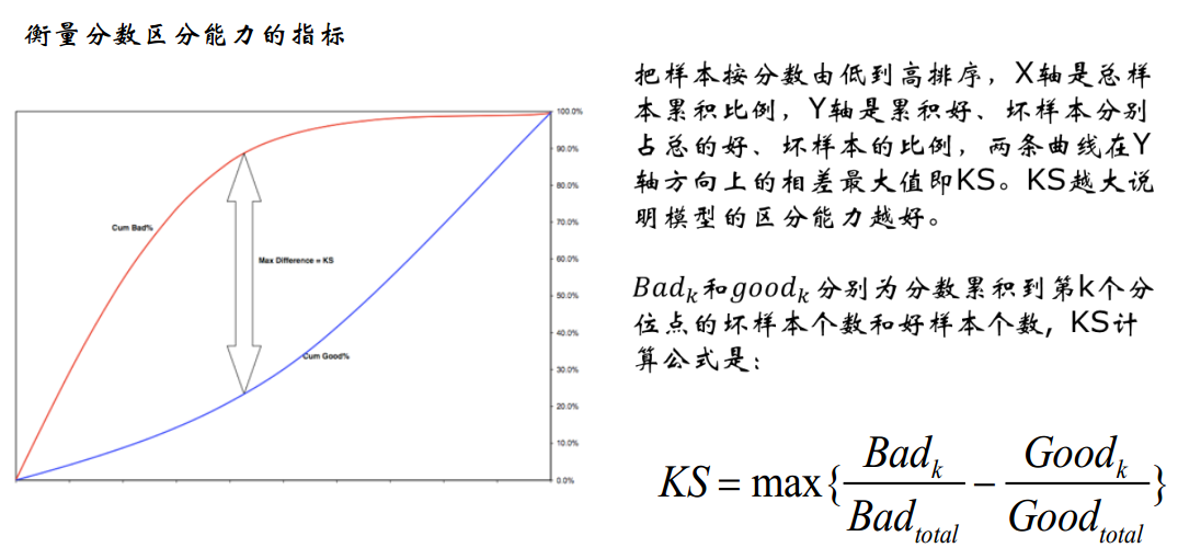
• 模型中用于区分预测正负样本分隔程度的评价指标，一般应用于金融风控领域。

• 与ROC曲线相似：

  • ROC是以FPR作为横坐标，TPR作为纵坐标，通过改变不同阈值，从而得到ROC曲线。

  • ks曲线为TPR-FPR，ks曲线的最大值通常为ks值。可以理解TPR是收益，FPR是代价，ks值是收益最大。图中绿色线是TPR、蓝色线是FPR。

KS的计算步骤如下：

1. 按照模型的结果对每个样本进行打分

2. 所有样本按照评分排序，从小到大分为10组（或20组）

3. 计算每个评分区间的好坏样本数。

4. 计算每个评分区间的累计好样本数占总好账户数比率(good%)和累计坏样本数占总坏样本数比率(bad%)。

5. 计算每个评分区间累计坏样本占比与累计好样本占比差的绝对值（累计bad%-累计good%），然后对这些绝对值取最大值即得此评分模型的K-S值。

注意：K-S值仅仅代表模型的分割样本的能力，不能表示分割的是否准确，即便好坏客户完全分错，K-S值依然可以很高

多分类问题

多分类时都一样，除了AUC

广告场景

CTR（Click-Through-Rate）

• 点击通过率,是互联网广告常用的术语,指网络广告（图片广告/文字广告/关键词广告/排名广告/视频广告等）的点击到达率,即该广告的实际点击次数（严格的来说,可以是到达目标页面的数量）除以广告的展现量(Show content). $\( ctr=\frac{点击次数}{展示量}　\tag{16} \)$

**CVR (Conversion Rate)，CVR即转化率。**是一个衡量CPA广告效果的指标

• 用户点击广告到成为一个有效激活或者注册甚至付费用户的转化率. $\( cvr=\frac{点击量}{转化量}　\tag{17} \)$

推荐场景

评估维度

• 覆盖率 = 指算法向用户推荐的文章占能符合露出条件文章的比例

• 多样性和新颖性：常见的问题是用户如果大量长时间的点击同一个主题或者是分类，其后推荐的资讯会呈现漏斗状，限制了用户的阅读。这时候就需要推荐系统进行猎奇的多样、新颖推荐以弥补这些缺陷

• 挖掘长尾的能力：推荐系统的一个重要价值就是发现长尾(长尾理论是 ChrisAnderson 提出的,不熟悉该理论的读者可以自行百度或者看 ChrisAnderson 出的《长尾理论》一书)，将小众的“标的物”分发给喜欢该类“标的物”的用户。度量出推荐系统挖掘长尾的能力，对促进长尾“标的物”的“变现”及更好地满足用户的小众需求从而提升用户的惊喜度非常有价值。

• 实时性：用户的兴趣是随着时间变化的，推荐系统怎么能够更好的反应用户兴趣变化，做到近实时推荐用户需要的“标的物”是特别重要的问题。

  • 特别像新闻资讯、短视频等满足用户碎片化时间需求的产品，做到近实时推荐更加重要。

• 响应及时稳定性：用户通过触达推荐模块，触发推荐系统为用户提供推荐服务，推荐服务的响应时长，推荐服务是否稳定(服务正常可访问，不挂掉)也是非常关键的。

指标

• ILS衡量推荐列表的多样性

  \(I L S(L)=\frac{\sum_{b_{i} \in L} \sum_{b_{j} \in L, b_{j}=b_{i}} S\left(b_{i}, b_{j}\right)}{\sum_{b_{i} \in L} \sum_{b_{j} \in L, b_{j}=b_{i}} 1}\)

  • \(S\left(b_{i}, b_{j}\right)\) 计算的是 \(i\) 和 \(j\) 两个物品的相似性

  • 如果推荐列表中的物品越不相似⇒ILS越小⇒推荐结果的多样性越好

• Hit Rate $\( \mathrm{HR}=\frac{\text { number of hits }}{\text { number of users }} \)$

  • #users是用户总 数, 而#hits是测试集中的item出现在Top- N推荐列表中的用户数量。

• Average Precision：在位置K的Average Precision用来衡量一个相关商品在所有ranks的精度。 $\( A P(R)_{k}=\frac{1}{\min (|R|, k)} \sum_{i=1}^{k} \delta(i \in R) \operatorname{Prec}(R)_{i} \)$

  def AP(ranked_list, ground_truth):
      """Compute the average precision (AP) of a list of ranked items
      ground_truth 表示是否正确的标识
      hits 表示 score （预测结果分值）倒排，从第0个到当前个的累计预测正确样本数
      sum_precs 表示每个 ground_truth = 1 的位置的 precision 的累加
      """
      hits = 0
      sum_precs = 0
      for n in range(len(ranked_list)):
          if ranked_list[n] in ground_truth:
              hits += 1
              sum_precs += hits / (n + 1.0)
      if hits > 0:
          return sum_precs / len(ground_truth)
      else:
          return 0
  

  • 那么对于MAP(Mean Average Precision)：所有用户 \(u\) 的AP再取均值

• Normalized Discounted Cummulative Gain(NDCG)

  • 累积增益CG，表示将每个推荐结果相关性的分值累加后作为整个推荐列表的得分。

    \(C G_{k}=\sum_{i=1}^{k} r e l_{i}\) , \(r e l_{i}\) 表示处于位置 \(i\) 的推荐结果的相关性, \(k\) 表示所要考察的推荐列表的大小

    缺点：

    • CG没有考虑每个推荐结果处于不同位置对整个推荐结果的影响，例如，我们总是希望相关性大的结果排在前面，相关性低的排在前面会影响用户体验。

  • DCG(Discounted Cummulative Gain)在CG的基础上引入了位置影响因素

    \(D C G_{k}=\sum_{i=1}^{k} \frac{2^{r e l_{i}}-1}{\log _{2}(i+1)}\)

    • 分子部分 \(2^{r e l_{i}}-1\)：\(r e l_{i}\) 越大, 即推荐结果 \(i\) 的相关性越大，推荐效果越好，DCG越大。

    • 分母部分 \(\log _{2}(i+1)\)：\(i\) 表示推荐结果的位置, \(i\) 越大, 则推荐结果在推荐列表中排名越靠后，推荐效果越差，DCG越 小。

    缺点：DCG针对不同的推荐列表之间很难进行横向评估，而我们评估一个推荐系统不可能仅使用一个用户的推荐列表及相应结果进行评估，而是对整个测试集中的用户及其推荐列表结果进行评估。

  • 那么，不同用户的推荐列表的评估分数就需要进行归一化，也就是NDCG。

• Mean Reciprocal Rank(MRR)

  \(M R R=\frac{1}{Q} \sum_{i=1}^{|Q|} \frac{1}{r a n k_{i}}\)

  • \(|Q|\) 是用户的个数, \(r a n k_{i}\) 是对于第 \(i\) 个用户, 推荐列表中第一个在ground-truth结果中的item所在的排列位置。

参考

1. 周志华 西瓜书

2. 李航 统计学习方法

3. https://baike.baidu.com/item/CVR/20215345

4. https://baike.baidu.com/item/CTR/10653699?fr=aladdin

5. https://www.cnblogs.com/shenxiaolin/p/9309749.html

6. https://www.cnblogs.com/wqbin/p/11105186.html

7. CSDN博主｜xiedelong｜推荐系统中的 MAP 评估指标

previous

因果推理方法

next

有监督学习